Measuring Fitness: Surge Prediction

Suppose it’s the final days of 2021. California’s Department of Public Health has asked us to predict the number of deaths due to COVID-19 that will occur over the next seven days. Our predictions will influence the policies that they pursue and the resources they request.

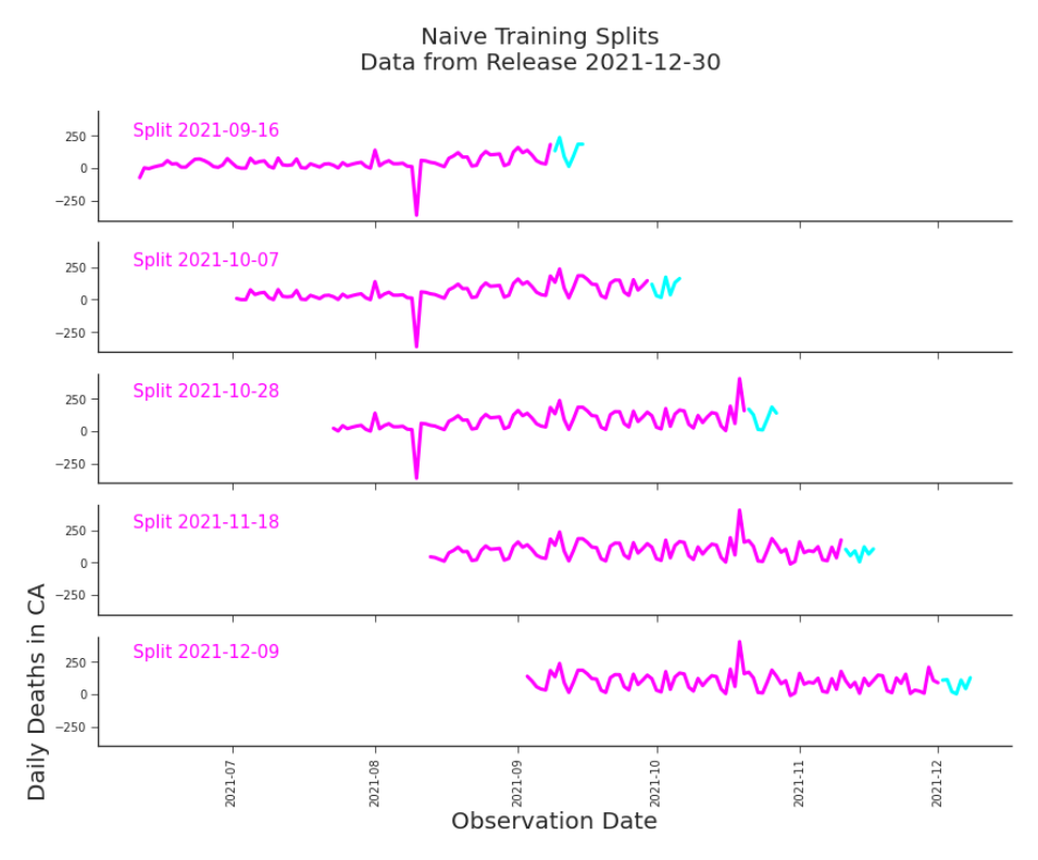
Figure 7.1. Training Splits for Time-Series Validation This design is intended to avoid the data leakage caused by training on future observation dates that standard cross validation incurs. However, it still suffers data leakage due to using a single release instead of training on the appropriate vintage data. We’re looking to build a simple autoregressive model. We propose to use the previous 90 days for training. Because we’re building a time series model, we

implement sliding window validation with five splits, each predicting 7 days and training on 90 days, as seen in Figure 7.1. After reviewing related research1 , we improve our validation method. Instead of training our model on only the current release, we use the history of releases, or the vintage data. We can see these splits in Figure 7.2. This will reduce our chances of getting a deceptively optimistic estimate of performance.

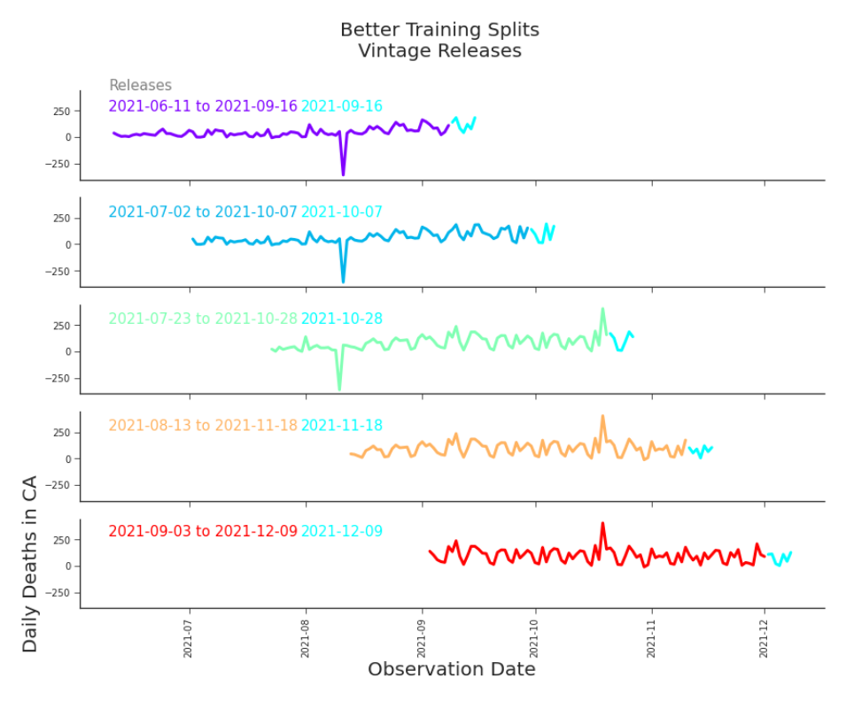
Figure 7.2. Training Splits for Time Series Validation, Using Vintage Data We improve the estimates of our sliding window validation by using the appropriate releases. Note, each split relies on multiple release for training data, although only the last is plotted for visual simplicity. Our raw data from JHU CSSE reports cumulative deaths, xii+1 , as we saw in

As discussed in 4.4.3.

j Chapter 6.2 In this use case we’re seeking to predict net new deaths, yij = xij − xi−1

where yij is the number of deaths that occurred on day i as reported on day j. Although the count of net new deaths seems straightforward enough, the recognition that data changes over time adds a new twist. When defining our labels, what release should be used to set the values for deaths on day i? We could use the latest available release, T , yTi . But that would treat values unequally, for the same reasons as discussed in Section 6.1. We i+k could choose the first released value, yi+1 i , or another consistent offset yi . How-

ever, we expect our work will be assessed according to the values reported on the last day of prediction, A prediction on day i will be judged on day i + 8, referring to release i + 7. So, we’ll set our prediction target to be values reported i+7 i+7 on that day: on day i we’ll predict yi+7 i , yi+1 , …, yi+6 . We’ll define our labels for

training accordingly. As shown in Figure 7.2, on day i + 1 we need the current release yi = [yi0 , yi1 , … , yii−1 ] = [x0i , x1i − x0i , … , xi−1 − xi−2 ]

as well as the prior releases, y1 , … , yi−1 . Fortunately, we are not equally impacted by data quality issues. The more time has passed since an issue occurred, the more we can control its effect through modeling choices. For example, if the December 30th, 2021 release is missing a value for May 1st, 2020, it may not have any effect on our modeling choices. However, if the same release is missing a value for December 28th, 2021, it will very likely impact our model and modeling choices. That is true for both older releases and older observations. Our measurements of data quality should reflect this diminishing impact of older

We are using the same underlying releases that we created in Chapter 6 and documented in the Appendix. The transformation to produce daily deaths and all other code for this chapter can be found in the Appendix.

issues. We are using the same dataset as we did in Chapter 6. We are applying it to the same broad problem (the COVID-19 pandemic). As such, we’ll rely on the same dimensions for data quality that we defined in Table 6.2. In general, relevant dimensions for data quality should be tailored to the data and application.

Accuracy

We need a measure of accuracy for a reported value. We’ve already done the legwork in Chapter 6 to identify that a value yij should be compared the value reported at κ releases into the future, yi+κ j . However, we may take another look at how we are comparing yij and yi+κ j . We could refer to our previous measure of accuracy, equation 6.1.4. However, our new use case has changed our needs. Previously, when measuring cumulative deaths we were not concerned about the edge cases of a 0 denominator. Now, as we are concerned with net new deaths, we hope that a 0 denominator-the truth value for net new deaths-is not an edge case. If we wanted to use our previous accuracy, we’d have to adapt it to accommodate the 0 denominator. But, we are no longer concerned about comparing the relative scale of errors across states. So, we can remove the denominator altogether, yi+κ j − y j , and still

preserve the direction of error. With this measurement of accuracy, we can now assess the accuracy of a release. Let’s measure a release i+1’s accuracy with a weighted average, giving heav123

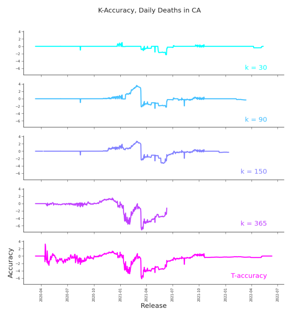
Figure 7.3. Accuracy of Releases, Daily Deaths in CA The accuracies of these releases follow similar patterns to our metric for accuracy in Figure 6.4. Notable differences appear on closer comparison and, of course, there is a dramatic change in scale.

ier weight to more recent observations,

α (κ) = Pi+1 i+1

On day i + 2, we cannot observe αi+1 (κ) because we won’t have the truth values for another κ days. We can only directly measure α j (κ) for j ≤ i + 1 − κ. We can use these observable values to estimate the accuracy of any release j, i + 2 − κ ≤ j ≤ i + 1. We can estimate αi+1 (κ) using α̂i+1 (κ) =

Estimation here, as in Chapter 6, is stymied by major restatements, as illustrated in Figure 7.3 and Figure 7.7. We don’t expect our accuracy predictions to perform well because we don’t assume that the revisions are predictable. Still, these estimates can be a useful signal to consider in the context of other DQ dimensions. We aren’t only concerned with the most recent release, though. We also need to understand the historic set of releases, which we’ll be relying on for training and testing. To assess the accuracy of all the available releases, we again take a weighted average, giving more weight to more recent releases  i+1  

Of course, on day i + 2 we can not observe all of these accuracies. Instead, we can estimate them using i+1−κ  

noting that α̂i (κ) = α̂ j (κ) ∀ j > i + 1 − κ. These estimates suffer the same obstacles as our previous estimates, as seen in Figure 7.4 and Figure 7.8.

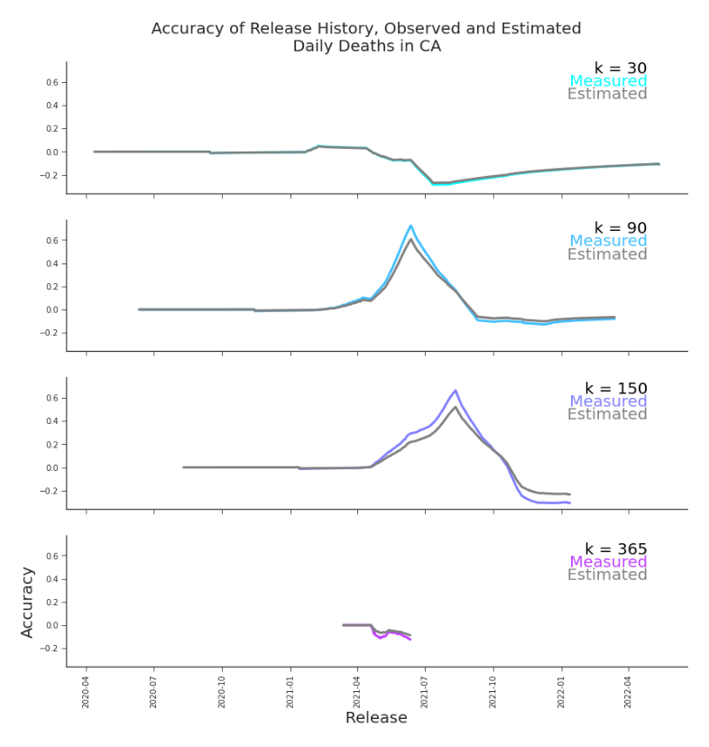
Figure 7.4. Accuracy of Release History, Observed and Estimated, Daily Deaths in CA The estimates of release history accuracy skews slightly more favorable than the observed values, but the trends align very closely. This owes not to predictability of errors but to the large overlap in summands.

Consistency

Predicting the future depends on learning from the past. An autoregressive model makes this explicit. Consistency determines how much of the past is usable. If the production process, measurement, or data definition change sufficiently, then data prior to the change will not be comparable to the data that is reported after it.

If that change is implemented backwards, rewriting history, we’ve termed it a retroactive change. A retroactive change, if it’s substantial enough, may constitute a major restatement. A major restatement may render the releases prior to the change no longer comparable to the subsequent ones. In practice, this means that our vintage data now begins with the major restatement. This puts the practitioner in a precarious position. Predictions that occur shortly after a major restatement, because they lack a depth of vintage data to train on, force the practitioner to either train without vintage data (and expect unreliably favorable performance estimates) or constrict the training set dramatically (and likely suffer model degradation as a result). If a change is only implemented for observations going forward, we call it a non-retroactive change. A non-retroactive change (NRC) divides observations within a release, making observations prior to the change no longer comparable to observations after it. An NRC that occurs as a first reported value doesn’t only make prior observations irrelevant, if persisted it will disqualify prior releases from our vintage dataset as well. Such an NRC essentially resets the data production process to day 0.

Let’s pretend that on December 1st, 2021, California changed how it counted deaths due to COVID-19. Previously, public health officials counted both probable and confirmed deaths towards the number of death due to COVID-19. With the change, they stopped counting probable deaths. Observations prior to December would measure something different than observations that occur going

forward. This would constitute a non-retroactive change. It should impact how we choose our data. Hopefully we can detect these sorts of changes in the data. When considering our usable data, we are concerned with the most recent NRC. Let the set of NRCs in a release i + 1 be i+1 i+1 Φi+1 = {ϕi+1 1 , … , ϕc } ϕ j ∈ {1, … , i}

where a non-retroactive change ϕi+1 indicates that the change occurred at yi+1 . j ϕi+1 j

Then, in release i + 1 the usable observations include ϕi+1 c to i. But, in this use case, we’re not only concerned with the most recent release, i + 1. We need to consider prior releases as well. So, we find the most recent shared, or common, NRC. Let’s consider the the multiset of non-retroactive changes that occur across releases 1 to i + 1, (Φi+1 , m) = {ϕm1 1 , … , ϕmc c }. The multiplicity, here indicated by the superscript m j , is constrained by m j ≤ i + 1 − ϕ j . That is, the number of times an observation appears in the multiset cannot exceed the number of times for which a value can be reported for an observation date by day i + 1. To consider a change common, we can say that it appears in at least α portion of possible releases,

Then, ηi+1 = max ϕ j s.t. 1{ ϕ j ∈Φi+1

identifies the most recent NRC across releases 1 to i + 1.

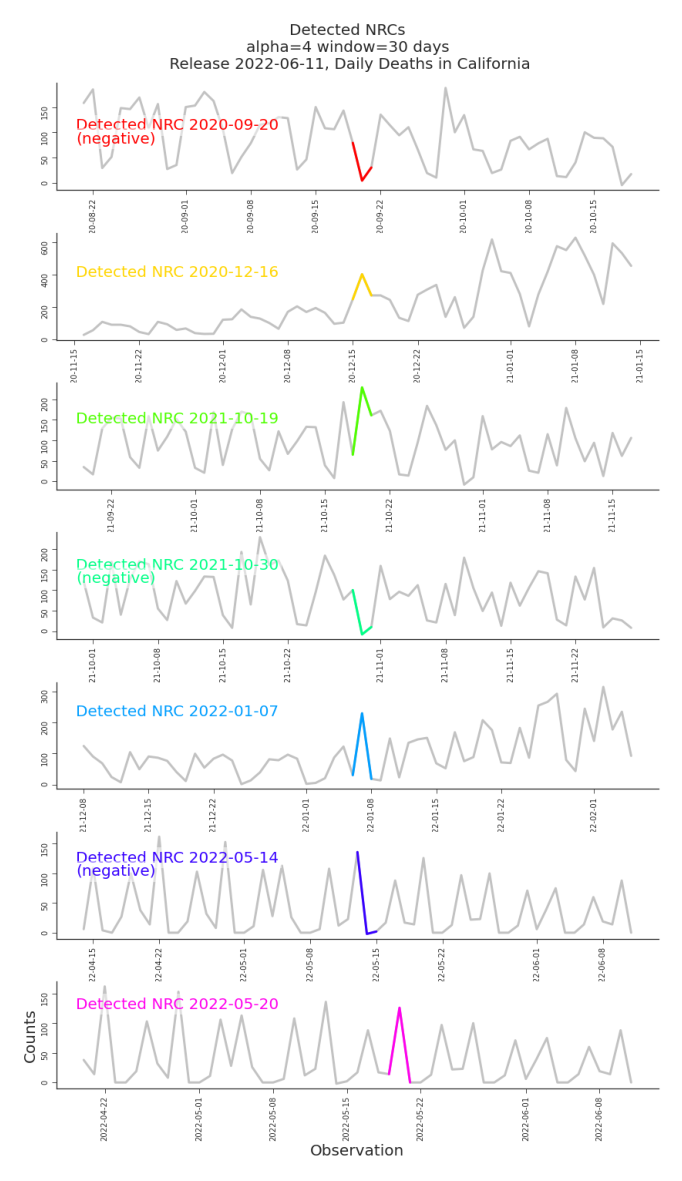
Figure 7.5. Detected Non-Retroactive Changes, Daily Deaths in CA Even our simple detection method is effective at identifying non-retroactive changes. Visual inspection reveals clear differences in cyclic patterns before and after the identified changes. Detail of the NRC on 2022-05-20 occurs in Figure 7.6.

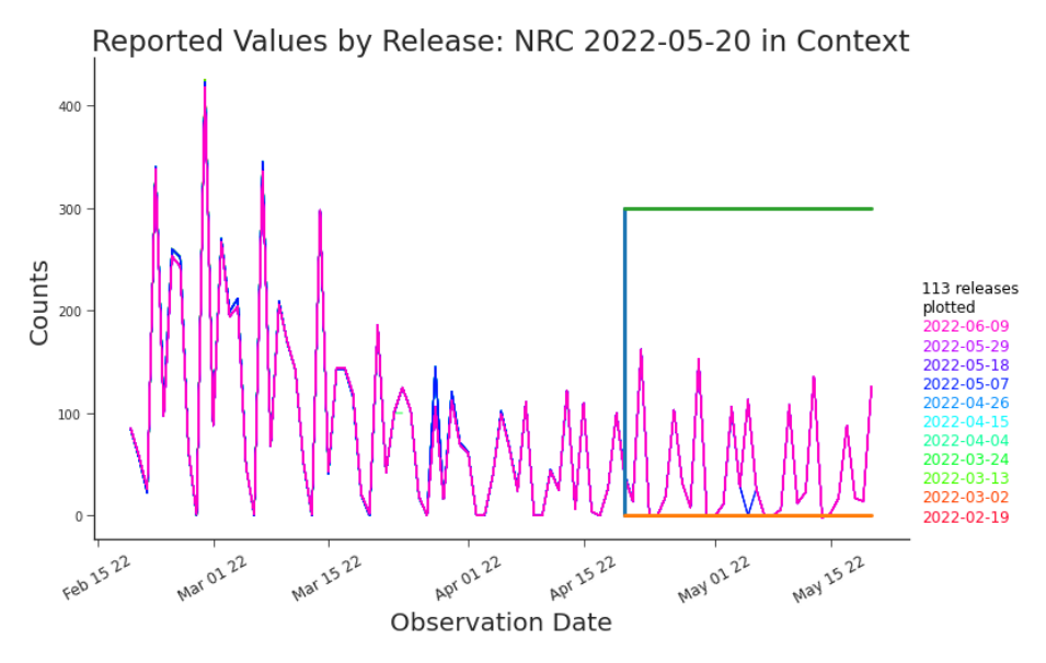
Figure 7.6. Detail of NRC on 2022-05-20 The box captures the window over which observation 2022-05-20 was evaluated as a non-retroactive change. We could argue that another NRC may have occurred near the left hand side of the box, near the 22nd of April, but was missed by our detection method. It’s worth considering the trade-offs of alternate modelling choices for NRC detection. Our pandemic data presents a challenge in identifying NRCs. We expect the data to reflect the true behavior of the pandemic, spikes and all. We’ve observed an artificial weekly cadence that distorts what we expect to be much a smoother underlying curve. In this case, a non-retroactive change does not need to divide samples from two neat distributions, as in change point detection, and any assumptions around the data being i.i.d or stationary would be in bad faith. The practical needs of NRC detection give us some direction. We’ll assume there are few non-retroactive changes relative to the true behavior and any artificial cadence introduced by reporting cycles. The costs of misclassifying an observation are also on our side. A false positive would unnecessarily shorten the history on which to train our model. A false negative would cause us to pos-

sibly train on historic data that we’d prefer not to. That is both undesirable and the current default behavior. Between the two, we’d prefer a false negative (the status quo) over a false positive. We must also consider the size of our data and the time constraints under which we need results. These constraints preclude methods that require attentive modeling, evaluation, or long run-times, ruling out many anomaly detection methods. We propose a modified z-score to accommodate both the lack of normality and the small sliding window which we assume to be relevant. We’ll adapt the score m to an online moving window estimator of size w, evaluating a new observation against the observations in the preceding window. Let W = [ j − w + 1, …, j] be the window of size w and ỹi+1 W the median of W. Define the median absolute deviations about the median i+1 i+1 MADi+1 W = median j∈W |y j − ỹW |.

i+1 yi+1 j+1 − ỹW

When MADi+1 W = 0, we calculate the modified z-score of observation j + 1 using i+1 yi+1

where i+1 i+1 MeanADi+1 W = avg j∈W |y j − ỹW |

is the mean absolute deviations about the median.

We have a second method of detecting NRCs: yi+1 j < 0. Any such value indicates that a change in what’s being reported may have occurred. We identify an observation j as representing an NRC in release i + 1 by j ∈ Φi+1 ⇐⇒ m( j + 1, i + 1, w) > α or yi+1 j < 0.

We can evaluate consistency due to NRCs at i + 1 using i − ηi+1 ,

the portion of consistent observations out of all possible observations.

Let’s suppose instead that on December 1st, when California changes how it counts deaths, it’s able to revise previously reported numbers. Starting with the December 1st release and going forward, all newly reported values will represent the number of confirmed deaths. All the releases prior to December 1st represent the sum of confirmed and probable deaths. All of these values are simply labelled ”deaths.” This would constitute a major restatement. If we are aware of it, it should impact how we use our data. A major restatement indicates that the data reported prior to the restatement is substantially different from the newly reported data. The last major restatement is the earliest release that contains data that is comparable to the data in David C. Hoaglin, 2013 suggests setting α to 3.5, although we’ve tuned it to a more conservative α = 4.

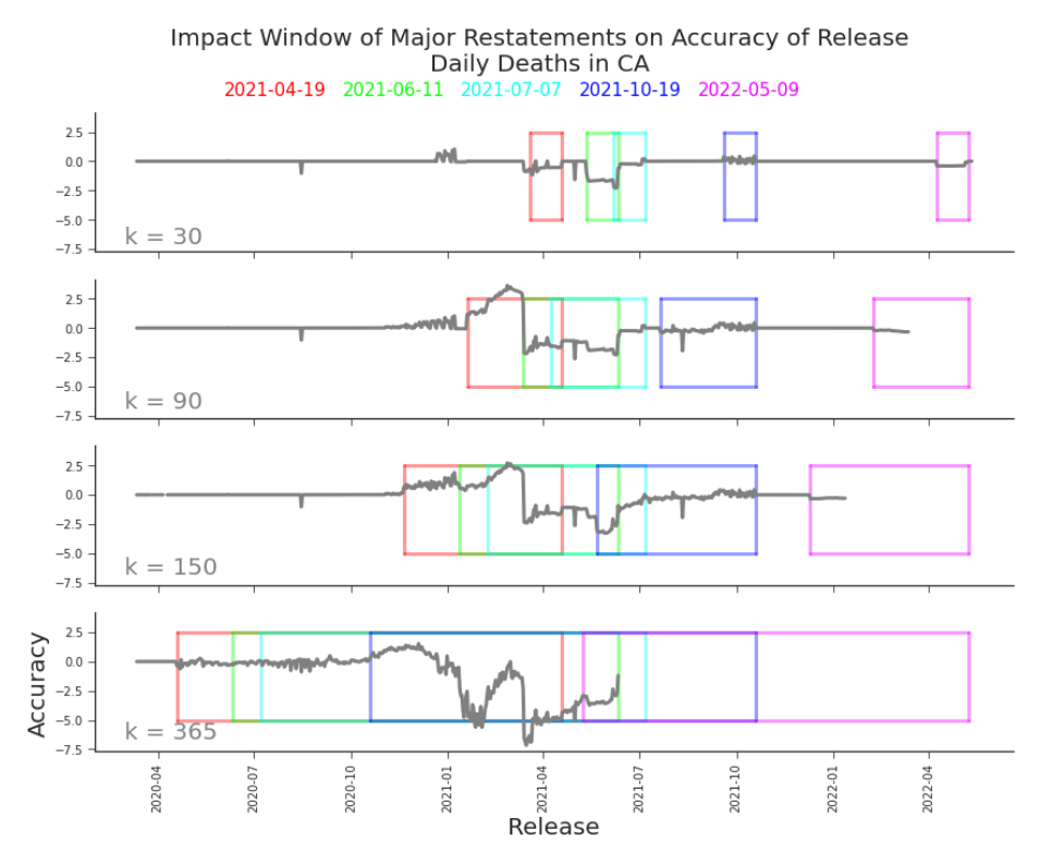
Figure 7.7. Impact of Major Restatements on Accuracy of Releases, Daily Deaths in CA We can investigate the impact of major restatements on accuracy, as we did in Figure 6.6. We see that, as before, major restatement windows capture changes in accuracy. our current release. Let the set of major restatements up to and including release i + 1 be ∆i+1 = {δ1 , … , δd }

where a major restatement is determined by a minimum portion of observations (β) that were changed more than a minimum threshold (α). For 2 ≤ k ≤ i + 1, k−1 i+1 1{|ykj − yk−1 j | > α} > β =⇒ k ∈ ∆ . k − 1 j=0

i+1 Then, δi+1 is the most recent major restatement. max , the maximum element of ∆

The number of usable releases is i + 1 − δi+1 max . We can measure consistency due to

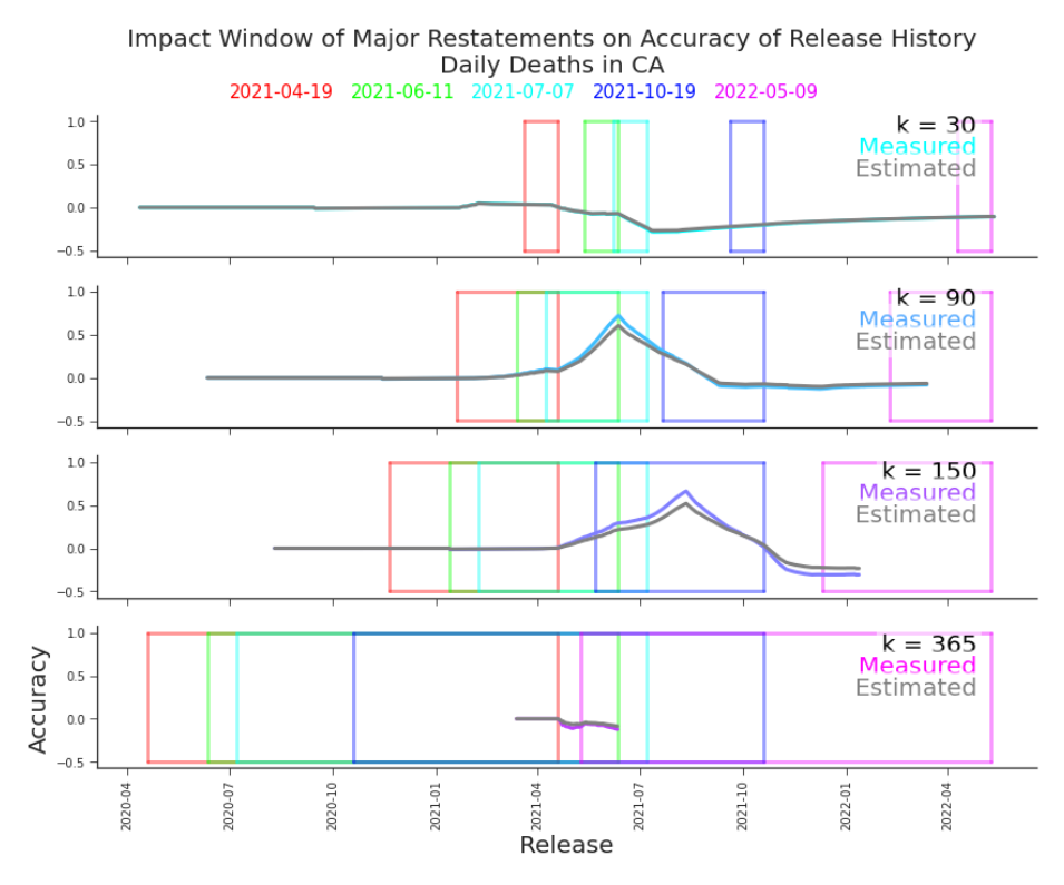
Figure 7.8. Impact of Major Restatements on Accuracy of Release History, Daily Deaths in CA Although still present, the connection between major restatements and accuracy of release history is less distinct than the accuracy of releases, as seen in Figure 7.7. major restatements as i + 1 − δi+1 max ,

the portion of consistent releases out of all possible releases.

Now that we’ve discussed NRCs and major restatements, we need to consider them in conjunction. We can lean on the heat maps that we introduced in Chap134

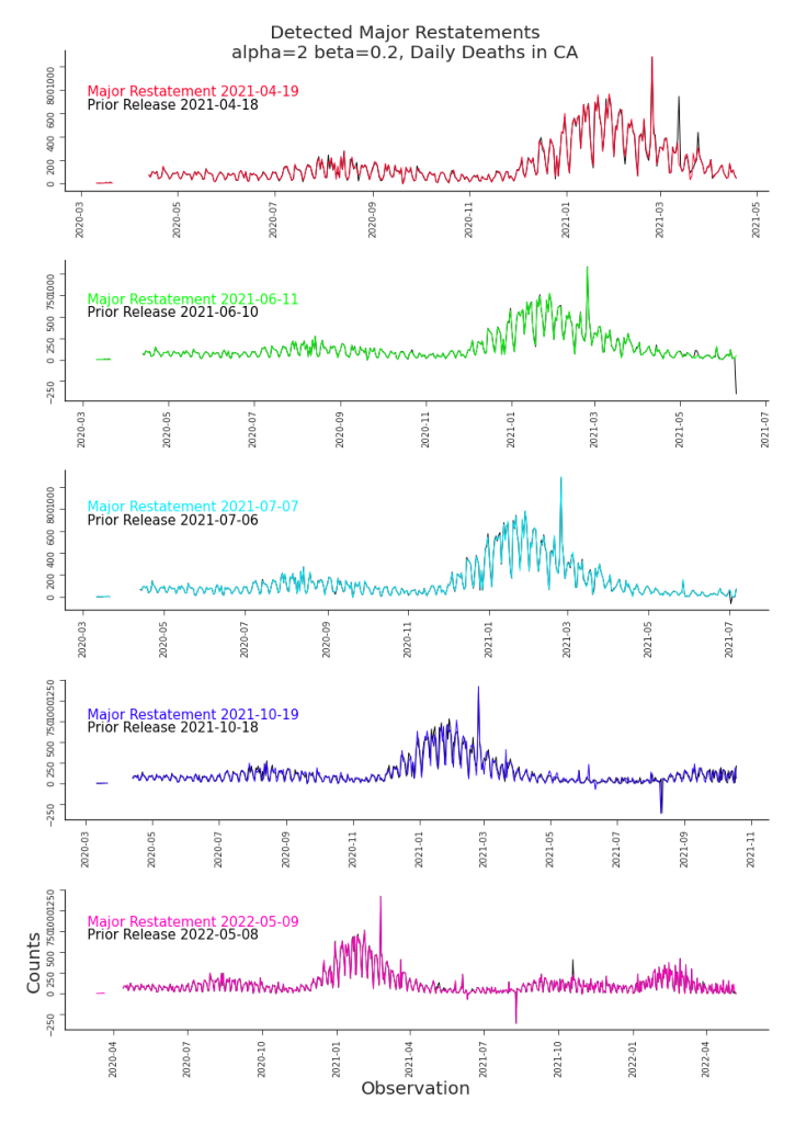
Figure 7.9. Detected Major Restatements, Daily Deaths in CA We’ve detected five major restatements but the changes introduced are difficult to appreciate in standard line plots. They are more effectively visualized in an impact plot, as seen in Figure 7.10.

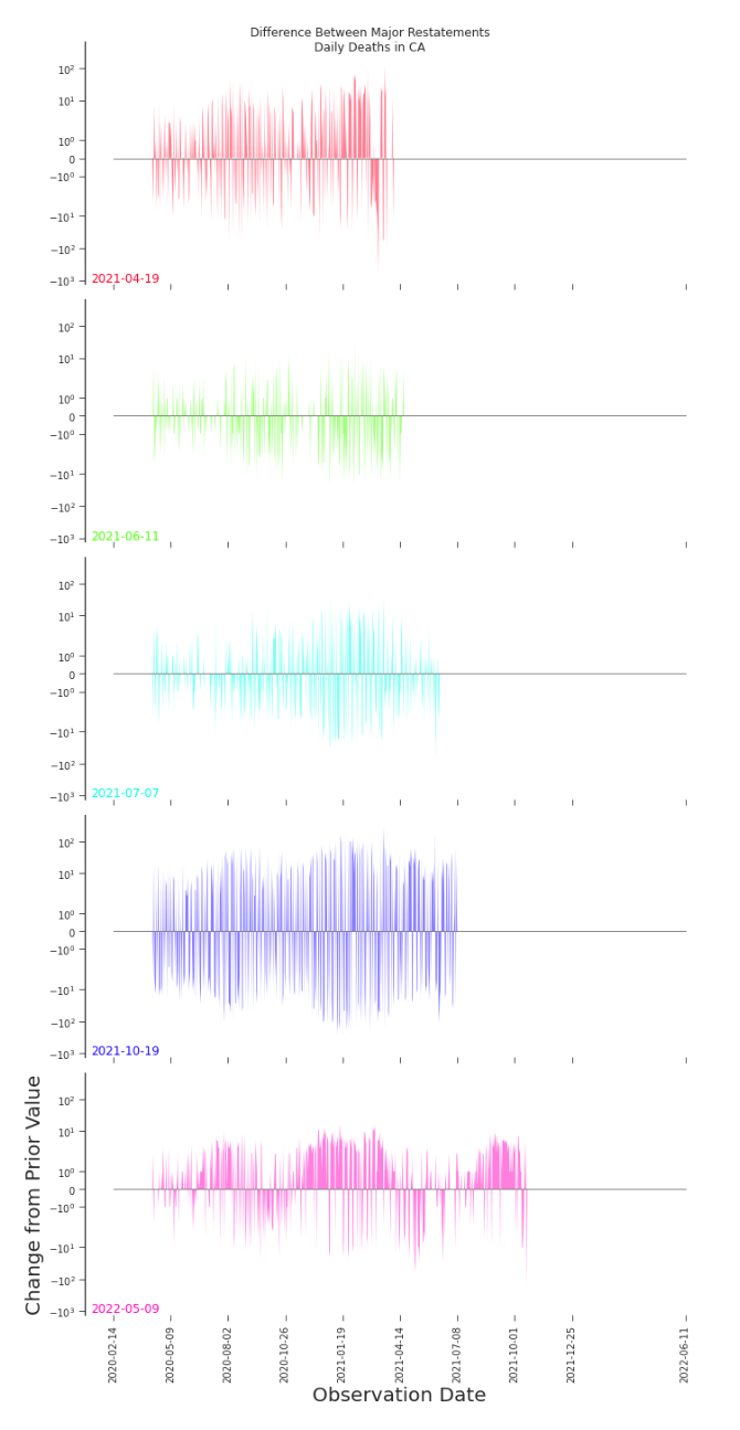
Figure 7.10. Impact Plot of Major Restatements, Daily Deaths in CA Using an impact plot, as introduced in Chapter 3, both the scale and trends of changes due to major restatements become much more apparent.

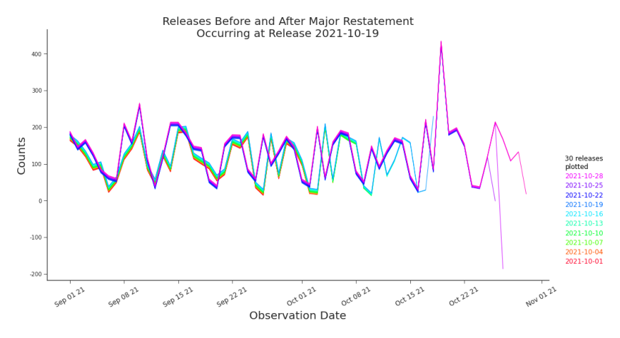
Figure 7.11. Shifted Line Plot Detail of Major Restatement on 2021-10-19 The ”bisected rainbow” shows the change in how releases report data before and after the restatement. On the right hand side we see the disruption caused by both the NRC and major restatement occurring at release 2021-10-18. ter 3 to plot common NRCs and major restatements (Figure 7.12). The uninterrupted horizontal stretches contain releases that are consistent with each other. The uninterrupted vertical spaces contain observations that are consistent with each other. Taken together, any area enclosed by vertical and horizontal bars (and above the diagonal) represent a set of consistent data. Our heat map (Figure 7.12) provides a guide to help us select what data to use when modeling.

Completeness

Suppose the number of deaths in California for May 1st, 2020 is missing. There was an outage in the computer system that day and the value will never be known. So, for all releases, it will always be missing. This is a very consequential issue on May 3rd, 2020. It’s not as consequential on May 3rd, 2023. The farther into history that a missing value occurs, the less damaging it is.

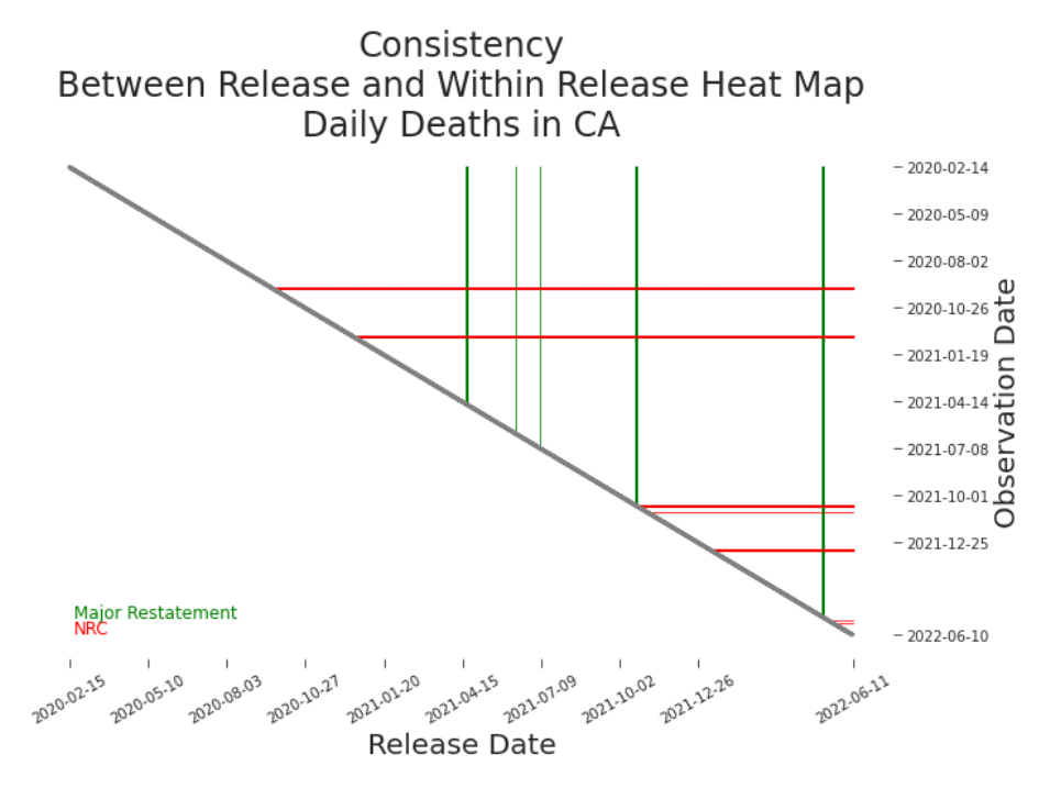
Figure 7.12. Between Release and Within Release Changes, Heat Map of Daily Deaths in CA By visualizing the NRCs and major restatements over our release history, it’s clear that we must use choose our data thoughtfully. The NRCs here are the same as those plotted in Figure 7.5. The major restatements are the same as those plotted in Figure 7.9. We need to measure completeness while acknowledging the decreasing impact of historic missing values. We measure the completeness of a release by weighing missing values inversely according to their distance into the past. i+1

Similarly, we measure the completeness of the data set at time i + 1 i+1 j × cj (i + 1)(i + 2) j=1

by penalizing missingness in earlier releases diminishingly harshly.

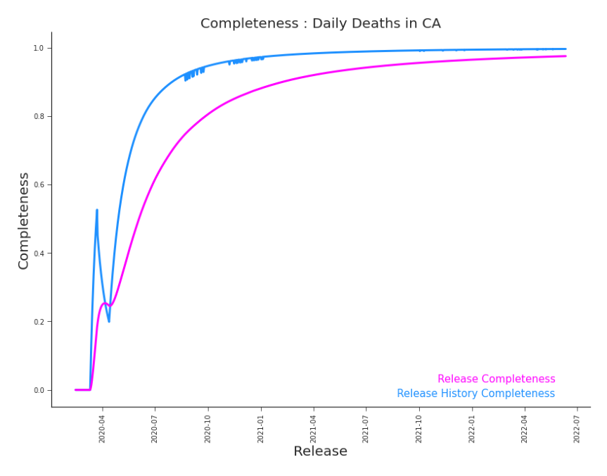
Figure 7.13. Completeness by Release and Release History, Daily Deaths in CA The impact of the large set of missing values from the beginning of the pandemic lingers, but it diminishes over time. These missing values can be seen in the horizontal black bar at the top of the plot in Figure 3.6.

Timeliness, Completeness, and Believability

Suppose you have built the dashboard that reports California deaths due to COVID-19. You notice that the data from April 4th, 2021 shows no new deaths on April 3rd. Then, again, the data from April 5th shows no new deaths for April 4th. It’s incredible–and a very abrupt change in deaths. It’s also wrong. And it’s soon to be corrected. Aggregate data and, in our case, data derived from aggregate data are particularly susceptible to hidden missingness. During data aggregation, having no reported values often yields a zero value (instead of a missing value). When this

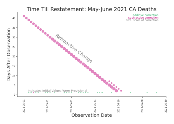
Figure 7.14. Reproduced Lag Plot, Cumulative Deaths in CA Reproduced here from Section 3.3, we can easily identify provisional values in a lag plot as a horizontal line. is the case, we call it an inferred zero. It assumes that the data production process is always working properly. But, we know that’s not the case. For example, data is often late. Let’s suppose that California wasn’t able to report the deaths for a given day in a timely fashion. Then, the golden state might be recorded as having zero deaths for that day.5 Unfortunately, that is indistinguishable in the data from a day when California actually has zero deaths. On the other hand, the data production process could have an affirmative zero requirement. In such a case, a state must report the number of deaths every day, whether or not there were any new deaths.6 California’s death count itself is an aggregation of the counties that comprise it. As such, California’s death count could conceal many missing values, even if there was an affirmative zero requirement, we would not know because standard practice is to aggregate the existing values. We discussed provisional data in Section 3.3 and explored it in Figure 3.14 and Figure 3.16. The latter is reproduced in Figure 7.14 for convenience. With a cu5

I.e., the cumulative death count would not increase. I.e., the cumulative death count did not change.

mulative count and no affirmative zero requirement, consistently late data ends up appearing as provisional data. That’s because the cumulative count from the prior day is used to fill-forward data that is late (and indistinguishable from a reported 0 new cases). In the case of cumulative deaths, it means yesterday’s death count is reported as today’s. In the case of net new deaths, it means a 0 value is reported, xii+1 = xii−1 =⇒ yi+1 =0. If values that are first reported as 0 are revised promptly, it calls into question whether those first reported values were actually reported or truly missing. These possibly late values challenge the believability of the data. We can assess this fill-forward lateness by estimating the probability that an observation with an initial value yi+1 = 0 will be promptly revised, within w days. We can estimate the probability that | yi+1 = 0) P(yi+1 = yi+2 = · · · = yi+1+w

by leveraging historic examples −1

where L = {y j+1 s.t. y j+1 = 0}. j j We could consider L a set of provisional changes, except we do not have a reasonable belief that these 0 values were truly reported. Indeed, they may be examples of hidden missingness.

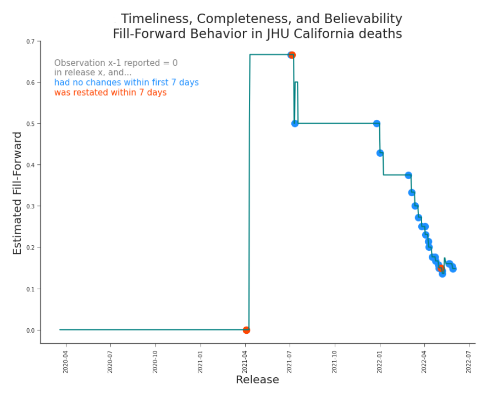
Figure 7.15. Assessing Fill-Forward Behavior, Daily Deaths in California Each observation that was first released as 0 impacts the fill-forward metrics 7 days after its first reported value. Note, even though most first-reported zero values were not promptly revised, it does not indicate they were reported accurately. This was calculated using Equation 7.4.1.

Validity and Believability

As we noted in our first use, cumulative deaths should not decrease. Likewise, net new deaths should not be negative. We can measure this directly, as soon as the data is published, using

1{yi+1 j < 0} .

This provides a simple and clean measurement of validity and believability for a single release.

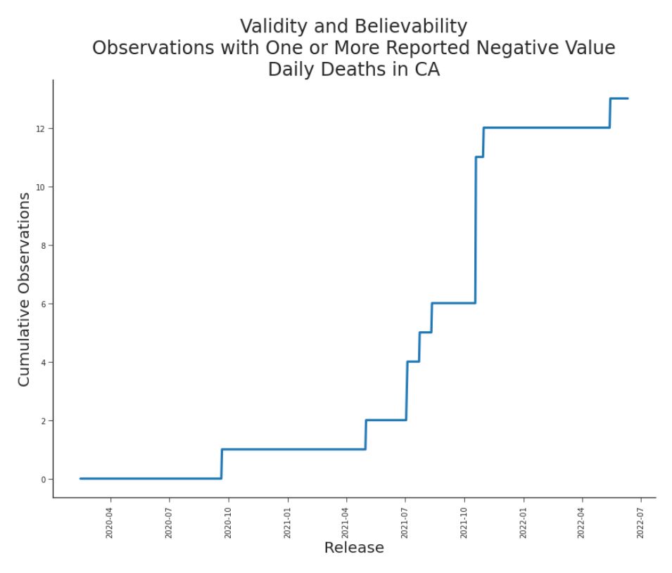
Figure 7.16. Validity and Believability, Daily Deaths in CA This metric should itself be non-decreasing, as each dataset contains the previous day’s dataset in its entirety. To assess the entire dataset, we’d prefer not to penalize consistency across releases. We can measure the validity and believability of the history of releases with j=1

1{ min ykj < 0} , k∈{1,…,i+1}

the number of observations that have been reported with a negative value in at least one release.

Believability

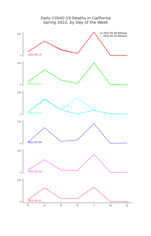
Figure 7.17. Reproduced Plot of Deaths by Day of the Week, CA See Figure 9 for full detail.

”Illness does not follow the seven-day week, but its record is defined by it.” Galaitsi et al., 2021

Suppose California began reporting deaths once a week, only on Mondays, and attributing all of the previous week’s deaths to Sunday. Then, according to the data, it would appear that people were waiting to die until Sunday. We

wouldn’t believe the data. Unbelievable as that sounds, it sounds familiar. In Section 0.5 we saw that, according to the data, most deaths in California were occurring on Tuesdays and Fridays (for a period of time). We explored the phenomenon in Figures 5 and 9. The latter is reproduced for convenience in Figure 7.17. It’s likely that there’s a combination of fill-forward behavior, inferred zeroes, and an unfortunate choice of reporting date attribution (see Chapter 2 for an exploration on the impact of reporting date choices). In order to evaluate our data, we need to detect whether there is this sort of suspicious preference to die on a particular weekday. We could refer to methods from time series analysis to detect the existence of a weekly seasonality. However, as discussed in Section 7.2.1 with NRC detection, we are constrained by the practical concerns of speed and scale. Also, we are more concerned with recent data quality than historic. In addition to older observations having had the chance to be revised, newer observations will impact predictions more heavily. We will assess whether or not there is a preference for attributing deaths to a particular day of the week, focusing on the most recently reported observations. To do this, we need to divide our data into weeks or, more precisely, sets of 7 consecutive days. Let S = {i − w7 + 1, … , i} be the set of recent observations and S v = {i − v7 − 6, i − v7 − 5, … , i − v7} v ∈ {0, … , w}

be the set of non-overlapping weeks.7 . Let S k = { j ∈ S and j mod 7 = k} be a set of observations all falling on the same day of the week. For convenience, let’s denote the seven-day window that observation j falls in as S 7 ( j), where = S 7 ( j) = S v for some v such that j ∈ S v . We will measure the believability of release i + 1 with a metric counting the number of strongly favored days of the week, b

1{median j∈S k P

Favoritism is determined by α ∈ (1/7, 1), the portion of a given week’s deaths above which must be attributed to a single day for that day to be considered favored. The range of bi+1 , the number of favored days, is determined by α.8 For example, α = 73 constrains bi+1 to a range of {0, 1, 2}. We’ve chosen the median over the mean for its robustness against outliers and one-off reporting errors.9 As we can see in Figure 7.18, this measurement readily identifies the suspicious weekly cadence observed in Figure 7.17.

Data Selection

Now, having taken a closer look at our data, we can revisit our prediction problem. Our metrics, as seen in Table 7.7, indicate we may want to reconsider the data that we’d originally chosen in Figure 7.2.

These are actually periods of 7 continuous days that do not, in general, align with calendar weeks.

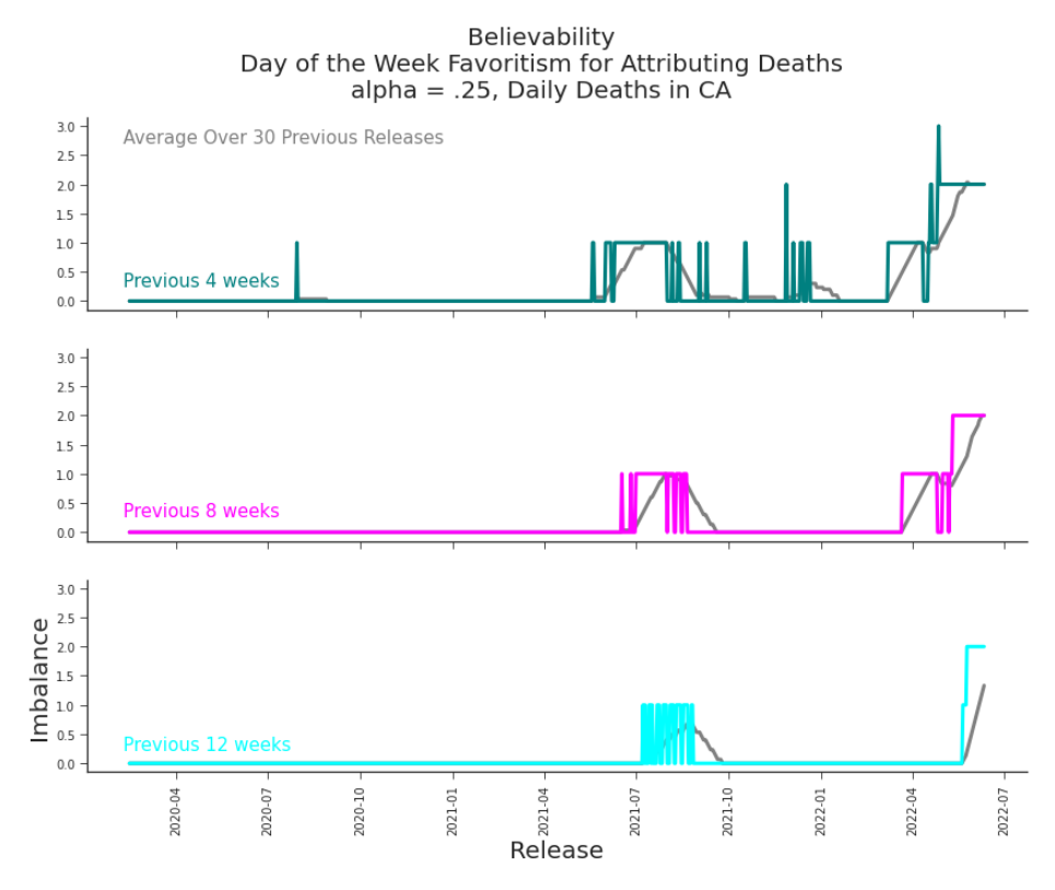
Figure 7.18. Favoritism for Attributing Deaths to a Day of the Week Our measurement readily identifies the two ’preferred’ weekdays to pass away on in May 2022. It also points us to a number of other concerns to investigate.

Table 7.1. Proposed Data Quality Dimensions for Surge Prediction

Dimensions	Target	Range	Goal	Eq.
Accuracy of Dataset	{y^1, …, y^(i+1)}	(−inf, inf)	0	7.1.3
Consistency MR	{y^1, …, y^(i+1)}	[0, 1]	1	7.2.4
Consistency NRC	{y^1, …, y^(i+1)}	[0, 1]	1	7.2.2
Completeness of Release	y^(i+1)	[0, 1]	1	7.3.1
Completeness of Dataset	{y^1, …, y^(i+1)}	[0, 1]	1	7.3.2
Timeliness, Completeness, and Believability	{y^1, …, y^(i+1)}	(0, 1)	1	7.4.1
Validity and Believability	{y^1, …, y^(i+1)}	{0, 1, …, i}	0	7.5.2
Believability of Release	y^(i+1)	{0, …, ⌊α⁻¹⌋}	0	7.6.1

Table 7.2. Real-Time DQ Assessment for Deaths in CA, Release 2021-10-19 First, we recall that here we’ve measured accuracy in the original units (deaths). The −0.15 score is actually fairly good. Our fill-forward metric is a bit damming, but it only applies to observations with 0 deaths as their first reported values (i such that yi+1 = 0), for which there are few. Our believability metric, which measures reporting day favoritism, indicates that although this release is not concerning, the recent releases might be. This means we should probably take a closer look at the vintage data we were planning to train on. The validity and believability metric, which indicates there are a good few days with negative deaths, should cause us to reconsider our modelling options. If we plot the detected non-retroactive changes, we see that our data undergoes quite a few of them (Figure 7.19). In fact, the most recent shared NRC occurred on October 19th, well into the observations that we had planned on using. Armed with knowledge about our the quality of our dataset, we are now able to make an informed decision about how we want to choose our data. We could be very conservative and choose consistency over the depth of history, as

	2021-12-30
Estimated Accuracy of Dataset, k = 30	-0.150
Consistency Major Restatement	0.107
Consistency Most Recent MR	2021-10-19
Consistency NRC	0.089
Consistency Most Recent NRC	2021-10-30
Completeness of Release	0.992
Completeness of Dataset	0.958
Timeliness, Completeness, and Believability	0.500
Validity and Believability	12
Believability of Release, alpha = .25, 4 weeks	0
Believability of Dataset, alpha = .25, 4 weeks, 30 release average	0.233

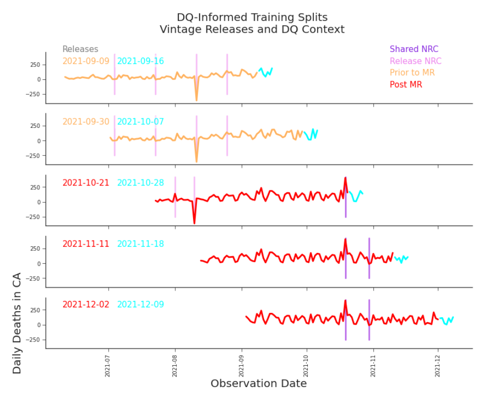
Figure 7.19. DQ-Informed Training Splits Using our data quality metrics, we are able to revisit our initial splits from Figures 7.1 and 7.2. We can see that our initial training data includes data that we have reason to believe is not directly comparable to the data we are aiming to predict. seen in Figure 7.20. If so, we would significantly decrease the size of our dataset, but we would be much more confident that our data has been produced by the same process that will yield our target values. However, this may reduce the size of our dataset drastically enough that it could result in reduced model performance. We should choose our candidate models in light of our data, taking care to include those that are robust against our data’s shortcomings. Likewise, we ought to choose our data with knowledge of its quality, balancing the trade-offs between data quality, data size, and model performance. Data

Table 7.3. Observed Accuracy, Daily Deaths in California, Release 2021-12-30 selection should occur independent of and prior to feature engineering and feature selection. It should be a thriving area of research and a practice as standard as model selection. Data quality should stand as the foundation upon which we prepare our data and build our models.

	Observed Accuracy, k = 30
2021-12-30	-0.154

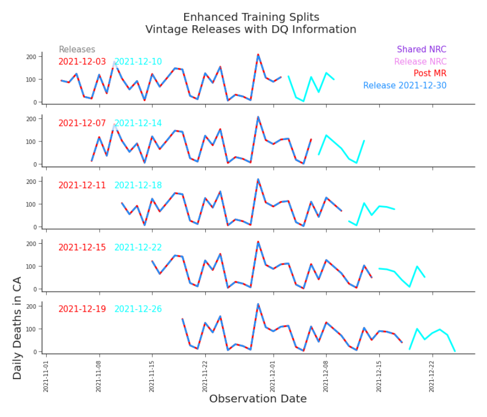
Figure 7.20. DQ-Informed Data Selection for Training Splits We have more confidence that this dataset is created by the same process that will produce the data we are predicting. But, it comes at the cost of reducing the size of the data significantly. We need to balance our quest for quality with our ability to train a model.

In the end, data selection is a modeling decision. It is an art, but one that would be greatly aided by a science. These past chapters have been an effort to lay a few bricks in the quantitative foundations of that science. Just as we opened Chapter 6, we’ll close this chapter. ”To become a science DQ must have a foundation built on measurement” (Karr, Sanil, and Banks, 2005).

---

Notes

2. ( j + 1) × (yi+1+κ − yi+1 j ) . j (i + 1)(i + 2) j=0 (7.1.1)

3. j   . j × α (κ)  (i + 1)(i + 2)  j=1

4. j i   j × α (κ) + α̂ (κ) j  (i + 1)(i + 2)  j=1 j=i+2−κ

5. j+1 − ỹW ×| | m( j + 1, i + 1, w) = 1.253314 MeanADi+1 W

6. The modified z score provides a more satisfying NRC detector than equation 3.2.3 used for visualization. Of course, the modified z score is suitable for filtering within releases changes in a heat map as well. 3

7. ( j + 1) × 1{xi+1 = j exists} . (i + 1)(i + 2) j=0

8. Note, bi+1 < 7. 9 In theory, we shouldn’t need to accommodate negative values, but in practice we’ve taken only the non-negative part of the summands.